6. Data Analysis Overview
The CYCLES samples recorded by the data collection subsystem tell us approximately how much total time was spent by each instruction at the head of the issue queue. However, when we see a large sample count for an instruction, we do not know immediately from the sample counts whether the instruction was simply executed many times or whether it stalled most of the times it was executed. In addition, if the instruction did stall, we do not know why. The data analysis subsystem fills in these missing pieces of information. Note that the analysis is done offline, after samples have been collected.
Given profile data, the analysis subsystem produces for each instruction:
For programs whose executions are deterministic, it is possible to measure the execution counts by instrumenting the code directly (e.g., using pixie). In this case, the first phase of the analysis, which estimates the frequency, is not necessary. However, many large systems (e.g., databases) are not deterministic; even for deterministic programs, the ability to derive frequency estimates from sample counts eliminates the need to create and run an instrumented version of the program, simplifying the job of collecting profile information.
The crux of the problem in estimating instruction frequency and cpi is that the sample data provides information about the total time spent by each instruction at the head of the issue queue, which is proportional to the product of its frequency and its cpi; we need to factor that product. For example, if the instruction's sample count is 1000, its frequency could be 1000 and its cpi 1, or its frequency could be 10 and its cpi 100; we cannot tell given only its sample count. However, by combining information from several instructions, we can often do an excellent job of factoring the total time spent by an instruction into its component factors.
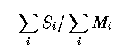
The bulk of the estimation process is focused on estimating the frequency, Fi, of each instruction i. Fi is simply the number of times the instruction was executed divided by the average sampling period, P, used to gather the samples. The sample count Si should be approximately FiCi, where Ci is the average number of cycles instruction i spends at the head of the issue queue. Our analysis first finds Fi; Ci is then easily obtained by division.
The analysis estimates the Fi values by examining one procedure at a time. The following steps are performed for each procedure:
The CFG is built by extracting the code for a procedure from the executable image. Basic block boundaries are identified from instructions that change control flow, e.g., branches and jumps. For indirect jumps, we analyze the preceding instructions to try to determine the possible targets of the jump. Sometimes this analysis fails, in which case the CFG is noted as missing edges. The current analysis does not identify interprocedural edges (e.g., from calls to longjmp), nor does it note their absence.
If the CFG is noted as missing edges, each block and each edge is assigned its own equivalence class. Otherwise, we use an extended version of the cycle equivalence algorithm in [JohPP94] to identify sets of blocks and edges that are guaranteed to be executed the same number of times. Each such set constitutes one equivalence class. Our extension to the algorithm is for handling CFG's with infinite loops, e.g., the idle loop of an operating system.
The heuristic for estimating the frequency of an equivalence class of instructions works on one class at a time. All instructions in a class have the same frequency, henceforth called F.
The heuristic is based on two assumptions: first, that at least some instructions in the class encounter no dynamic stalls, and second, that one can statically compute, for most instructions, the minimum number of cycles Mi that instruction i spends at the head of the issue queue in the absence of dynamic stalls.
Mi is obtained by scheduling each basic block using a model of the processor on which it was run. Mi may be 0. In practice, Mi is 0 for all but the first of a group of multi-issued instructions. An issue point is an instruction with Mi > 0.
If issue point i has no dynamic stalls, the frequency F should be, modulo sampling error, Si / Mi. If the issue point incurs dynamic stalls, Si will increase. Thus, we can estimate F by averaging some of the smaller ratios Si / Mi of the issue points in the class.
As an example, Figure 7 illustrates the analysis for the copy loop
shown previously in Figure 2.
The Mi column shows the output from the instruction
scheduler, and the Si / Mi column shows
the ratio for each issue point. The heuristic used various rules to
choose the ratios marked with * to be averaged, computing
a frequency of 1527. This is close to 1575.1, the true frequency for
this example.
Addr   Instruction           Si    Mi   Si / Mi
009810 ldq    t4, 0(t1)     3126   1     3126
009814 addq   t0, 0x4, t0      0   0
009818 ldq    t5, 8(t1)     1636   1     1636
00981c ldq    t6, 16(t1)     390   0
009820 ldq    a0, 24(t1)    1482   1     1482 *
009824 lda    t1, 32(t1)       0   0
009828 stq    t4, 0(t2)    27766   1    27766
00982c cmpult t0, v0, t4       0   0
009830 stq    t5, 8(t2)     1493   1     1493 *
009834 stq    t6, 16(t2)  174727   1   174727
009838 stq    a0, 24(t2)    1548   1     1548 *
00983c lda    t2, 32(t2)       0   0
009840 bne    t4, 0x009810  1586   1     1586 *
There are several challenges in making accurate estimates. First, an equivalence class might have few issue points. In general, the smaller the number of issue points, the greater the chance that all of them encounter some dynamic stall. In this case, the heuristic will overestimate F. At the extreme, a class might have no issue points, e.g., because it contains no basic blocks. In this case, the best we can do is exploit flow constraints of the CFG to compute a frequency in the propagation phase.
Second, an equivalence class might have only a small number of samples. In this case, we estimate F as:
Third, Mi may not be statically determinable. For
example, the number of cycles an instruction spends at the head of the
issue queue may in general depend on the code executed before the
basic block. When a block has multiple predecessors, there is no one
static code schedule for computing Mi. In this
case, we currently ignore all preceding blocks. For the block listed
in Figure 7, this limitation leads to an error: Mi
for the ldq instruction at 009810 should be 2 instead of
1 because the processor cannot issue a ldq two cycles
after the stq at 009838 from the previous iteration.
Thus, a static stall was misclassified as a dynamic stall and the
issue point was ignored.
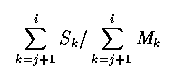
Fourth, dynamic stalls sometimes make the Mi values inaccurate. Suppose an issue point instruction i depends on a preceding instruction j, either because i uses the result of j or because i needs to use some hardware resource also used by j. Thus, Mi is a function of the latency of j. If an instruction between j and i incurs a dynamic stall, this will cause i to spend fewer than Mi cycles at the head of the issue queue because the latency of j overlaps the dynamic stall. To address this problem, we use the ratio:
Finally, one must select which of the ratios to include in the average. In rough terms, we examine clusters of issue points that have relatively small ratios, where a cluster is a set of issue points that have similar ratios (e.g., maximum ratio in cluster <= 1.5 * minimum ratio in cluster). However, to reduce the chance of underestimating F, the cluster is discarded if its issue points appear to have anomalous values for Si or Mi, e.g., because the cluster contains less than a minimum fraction of the issue points in the class or because the estimate for F would imply an unreasonably large stall for another instruction in the class.
Local propagation exploits flow constraints of the CFG to make additional estimates. Except for the boundary case where a block has no predecessors (or successors), the frequency of a block should be equal to the sum of the frequencies of its incoming (or outgoing) edges.
The flow constraints have the same form as dataflow equations, so for this analysis we use a variant of the standard, iterative algorithm used in compilers. The variations are (1) whenever a new estimate is made for a block or an edge, the estimate is immediately propagated to all of the other members in the block or edge's equivalence class, and (2) no negative estimates are allowed. (The flow equations can produce negative values because the frequency values are only estimates.) Because of the nature of the flow constraints, the time required for local propagation is linear in the size of the CFG.
We are currently experimenting with a global constraint solver to adjust the frequency estimates where they violate the flow constraints.
The analysis uses a second heuristic to predict the accuracy of each frequency estimate as being low, medium, or high confidence. The confidence of an estimate is a function of the number of issue points used to compute the estimate, how tightly the ratios of the issue points were clustered, whether the estimate was made by propagation, and the magnitude of the estimate.
A natural question at this point is how well the frequency estimates produced by our tools match the actual frequencies. To evaluate the accuracy of the estimates, we ran a suite of programs twice: once using the profiling tools, and once using dcpix, a pixie-like tool that instruments both basic blocks and edges at branch points to obtain execution counts. We then compared the estimated execution counts FP, where F is the frequency estimate and P the sampling period, to the measured execution counts -- the values should be approximately equal (modulo sampling error) for programs whose execution is deterministic.
For this experiment, we used a subset of the SPEC95 suite. The subset contains the "base" versions of all floating point benchmarks, and the "peak" versions of all integer benchmarks except ijpeg. The other executables lacked the relocation symbols required by dcpix, and the instrumented version of ijpeg did not work. The profiles were generated by running each program on its SPEC95 workload three times.
Figure 8 is a histogram showing the results for instruction frequencies. The x-axis is a series of sample buckets. Each bucket covers a range of errors in the estimate, e.g., the -15% bucket contains the samples of instructions where FP was between .85 and .90 times the execution count. The y-axis is the percentage of all CYCLES samples.
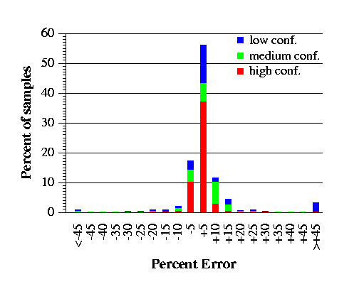
As the figure shows, 73% of the samples have estimates that are within 5% of the actual execution counts; 87% of the samples are within 10%; 92% are within 15%. Furthermore, nearly all samples whose estimates are off by more than 15% are marked low confidence.
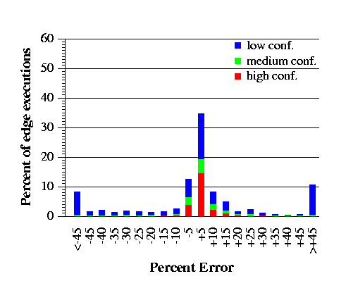
Figure 9 is a measure of the accuracy of the frequency estimates of edges. Edges never get samples, so here the y-axis is the percentage of all edge executions as measured by dcpix. As one might expect, the edge frequency estimates, which are made indirectly using flow constraints, are not as accurate as the block frequency estimates. Still, 58% of the edge executions have estimates within 10%.
To gauge how the accuracy of the estimates is affected by the number of CYCLES samples gathered, we compared the estimates obtained from a profile for a single run of the integer workloads with those obtained from 80 runs. For the integer workloads as a whole, results in the two cases are similar, although the estimates based on 80 runs are somewhat more tightly clustered near the -5% bucket. E.g., for a single run, 54% of the samples have estimates within 5% of the actual execution counts; for 80 runs, this increases to 70%. However, for the individual programs such as gcc on which our analysis does less well using data from a small number of runs, the estimates based on 80 runs are significantly better. With a single run of the gcc workload, only 23% of the samples are within 5%; with 80 runs, this increases to 53%.
Even using data from 80 runs, however, the > 45% bucket does not get much smaller for gcc: it decreases from 21% to 17%. We suspect that the samples in this bucket come from frequency equivalence classes with only one or two issue points where dynamic stalls occur regularly. In this case, gathering more CYCLES samples does not improve the analysis.
The analysis for estimating frequencies and identifying culprits is relatively quick. It takes approximately 3 minutes to analyze the suite of 17 programs, which total roughly 26MB of executables. Roughly 20% of the time was spent blocked for I/O.
Identifying which instructions stalled and for how long reveals where the performance bottlenecks are, but users (and, eventually, automatic optimizers) must also know why the stalls occurred in order to solve the problems. In this section, we outline the information our tools offer, how to compute it, and how accurate the analysis is.
Our tools provide information at two levels: instruction and procedure. At the instruction level, we annotate each stall with culprits (i.e., possible explanations) and, if applicable, previous instructions that may have caused the stall. Culprits are displayed as labeled bubbles between instructions as previously shown in Figure 2. For example, the analysis may indicate that an instruction stalled because of a D-cache miss and point to the load instruction fetching the operand that the stalled instruction needs. At the procedure level, we summarize the cycles spent in the procedure, showing how many have gone to I-cache misses, how many to D-cache misses, etc., by aggregating instruction-level data. A sample summary is shown earlier in Figure 4. With these summaries, users can quickly identify and focus their effort on the more important performance issues in any given procedure.
For each stall, we list all possible reasons rather than a single culprit because reporting only one culprit would often be misleading. A stall shown on the analysis output is the average of numerous stalls that occurred during profiling. An instruction may stall for different reasons on different occasions or even for multiple reasons on the same occasion. For example, an instruction at the beginning of a basic block may stall for a branch misprediction at one time and an I-cache miss at another, while D-cache misses and write-buffer overflow may also contribute to the stall if that instruction stores a register previously loaded from memory.
To identify culprits for stalls, we make use of a variety of information. Specifically, we need only the binary executable and sample counts for CYCLES events. Sample counts for other types of events are taken into consideration if available, but they are optional. Source code is not required. Neither is symbol table information, although the availability of procedure names would make it easier for users to correlate the results with the source code.
Our analysis considers both static and dynamic causes of stalls. For static causes, we schedule instructions in each basic block using an accurate model of the processor issue logic and assuming no dynamic stalls. Detailed record-keeping provides how long each instruction stalls due to static constraints, why it stalls, and which previously issued instructions may cause it to stall. These explain the static stalls. Additional stall cycles observed in the profile data are treated as dynamic stalls.
To explain a dynamic stall at an instruction, we follow a "guilty until proven innocent" approach. Specifically, we start from a list of all possible reasons for dynamic stalls in general and try to rule out those that are impossible or extremely unlikely in the specific case in question. Even if a candidate cannot be eliminated, sometimes we can estimate an upper bound on how much it can contribute to the stall. When uncertain, we assume the candidate to be a culprit. In most cases, only one or two candidates remain after elimination. If all have been ruled out, the stall is marked as unexplained, which typically accounts for under 10% of the samples in any given procedure (8.6% overall in the entire SPEC95 suite). The candidates we currently consider are I-cache misses, D-cache misses, instruction and data TLB misses, branch mispredictions, write-buffer overflows, and competition for function units, including the integer multiplier and floating point divider. Each is ruled out by a different technique. We illustrate this for I-cache misses.
The key to ruling out I-cache misses is the observation that an instruction is extremely unlikely to stall due to an I-cache miss if it is in the same cache line as every instruction that can execute immediately before it. (Even so, an I-cache miss is still possible in some scenarios: the stalled instruction is executed immediately after an interrupt or software exception returns, or the preceding instruction loads data that happen to displace the cache line containing the stalled instruction from a unified cache. These scenarios are usually rare.) More specifically, we examine the control flow graph and the addresses of instructions. If a stalled instruction is not at the head of a basic block, it can stall for an I-cache miss if and only if it lies at the beginning of a cache line. If it is at the head of a basic block, however, we can determine from the control flow graph which basic blocks may execute immediately before it. If their last instructions are all in the same cache line as the stalled instruction, an I-cache miss can be ruled out. For this analysis, we can ignore basic blocks and control flow edges executed much less frequently than the stalled instruction itself.
If IMISS event samples have been collected, we can use them to place an upper bound on how many stall cycles can be attributed to I-cache misses. Given the IMISS count on each instruction and the sampling period, we estimate how many I-cache misses occurred at any given instruction. From this estimate and the execution frequency of the instruction, we then compute the upper bound on stall cycles by assuming pessimistically that each I-cache miss incurred a cache fill all the way from memory.
How accurate is the analysis? Since in any nontrivial program there is often no way, short of detailed simulation, to ascertain why individual instructions stalled, we cannot validate our analysis directly by comparing its results with some "correct" answer. Instead, we evaluate it indirectly by comparing the number of stall cycles it attributes to a given cause with the corresponding sample count from event sampling, which serves as an alternative measure of the performance impact of the same cause. Though not a direct quantitative metric of accuracy, a strong correlation would suggest that we are usefully identifying culprits. (Since events can have vastly different costs, even exact event counts may not produce numbers of stall cycles accurate enough for a direct comparison. For example, an I-cache miss can cost from a few to a hundred cycles, depending on which level of the memory hierarchy actually has the instruction.) Again, we illustrate this validation approach with I-cache misses.
Figure 10 plots I-cache miss stall cycles against IMISS events for the procedures accounting for 99.9% of the execution time of each benchmark in the SPEC95 suite, with part of the main graph magnified for clarity. Each of the 1310 procedures corresponds to a vertical bar. The x-axis is the projected number of I-cache misses in that procedure, calculated by scaling the IMISS counts by the sampling period. The y-axis is the number of stall cycles attributed to I-cache misses by our tools, which report a range because some stall cycles may be caused only in part by I-cache misses. (To isolate the effect of culprit analysis from that of frequency estimation in this experiment, the analysis used execution counts measured with instrumented executables as described in Section 6.2.)
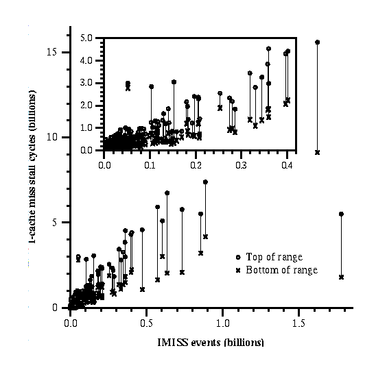
Figure 10 shows that the stall cycles generally
increase with the IMISS counts, with each set of endpoints clustering around
a straight line except for a few outlier pairs.
In more quantitative terms, the
correlation coefficients between the IMISS count of each procedure and
the top, bottom, and midpoint of the corresponding range of stall cycles are
0.91, 0.86, and 0.90 respectively, all suggesting a strong (linear)
correlation. We would expect some points to deviate substantially from the
majority because the cost of a cache miss can vary widely and our analysis
is heuristic. For example, Figure 10 has two
conspicuous outliers near (0.05,3) and (1.8,4). In the first case, the
number of stall cycles is unusually large because of an overly pessimistic
assumption concerning a single stall in the compress benchmark of SPECint95.
In the second case, the number is smaller than expected because the
procedure (twldrv in fpppp of
SPECfp95) contains long basic blocks,
which make instruction prefetching especially effective, thus reducing
the penalty incurred by the relatively large number of cache misses.
Beginning of paper
Abstract
1. Introduction
2. Related Work
3. Data Analysis Examples
4. Data Collection System
5. Profiling Performance
6. Data Analysis Overview
7. Future Directions
8. Conclusions
Acknowledgements
References